![]()
![]() Study Methods
Study Methods ![]()

H. J. Andrews Experimental Forest, OR
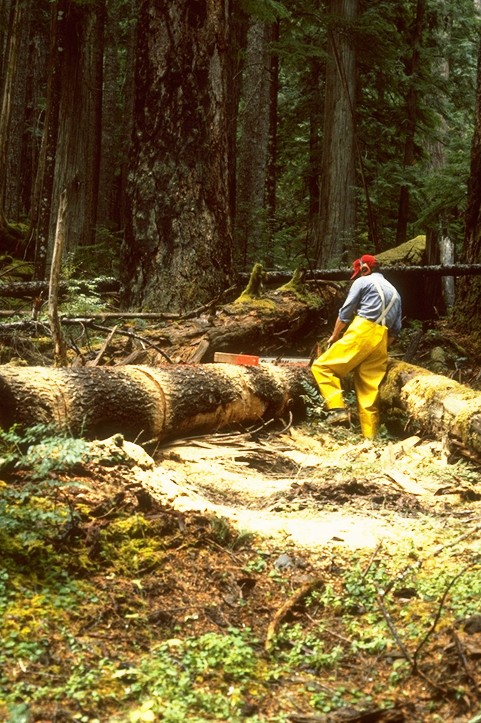
Cutting samples from a log
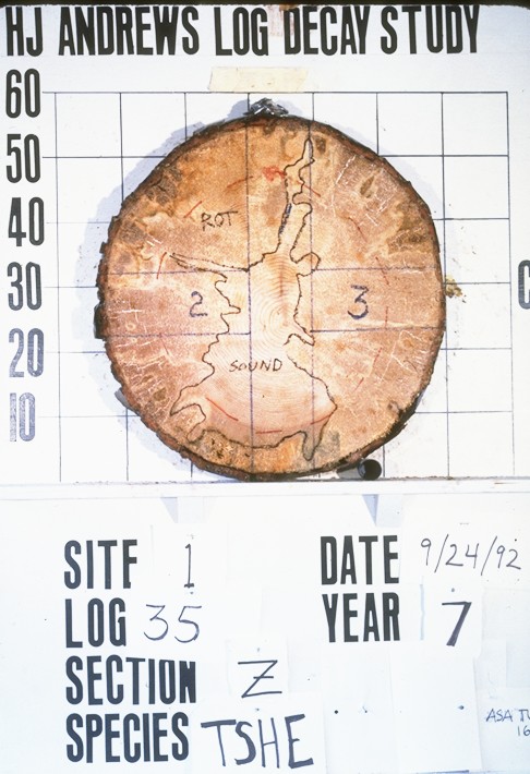
Cross-section from 7 year old Tsuga
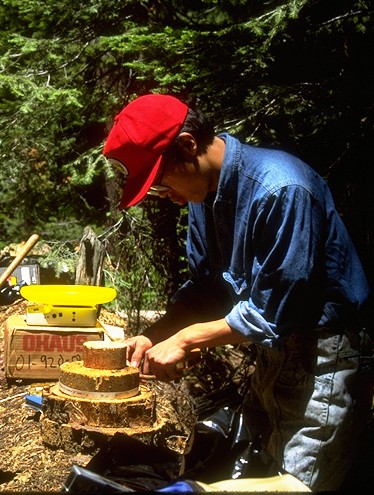
Measuring outer diameter
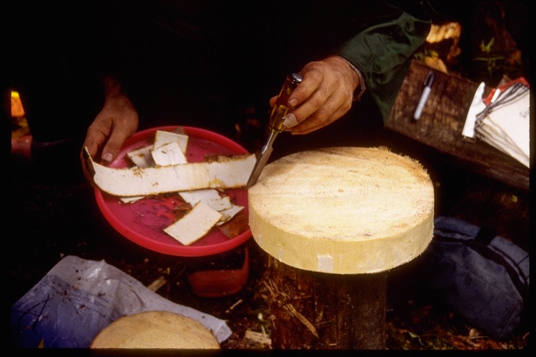
Removing bark from the sample
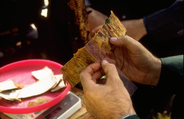
Measuring longitudinal thickness of bark
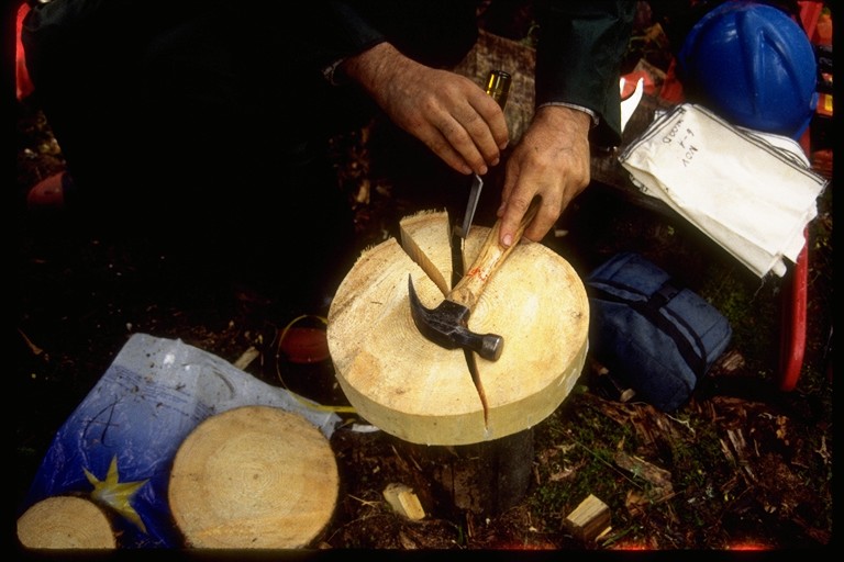
Cutting out a sub-sample for moisture content
General methods in determining decomposition rates
The general approach used at each of the sites differed (Table 2). The three methods used, chronosequence, time series, and decomposition vectors are defined below.
Chronosequence
Approach. The chronosequence approach was used at Fraser, Frissell ridge,
Klamath, and Sequoia to
determine decomposition rates from logs in which the sampling occurred
only once. In a
chronosequence one ages many pieces in various states of decay and
examines how a parameter such as density changes through time.
This is a substitution of space for time, and while not as precise
as a time series experiment (where individual pieces are followed through
time) it provides a good first approximation of decomposition rates
(Harmon et al. 1998).
Time
Series.
In a time series a cohort of fresh logs is placed out and
individual pieces are followed through time (Harmon et al .1998).
Typically a log is sampled once, after a planned interval expires.
As different logs are sampled over time the trend in decomposition
is revealed. It is more
accurate than the chronosequence approach, but takes a great deal more
time to examine the full range of changes.
This method was used at H. J. Andrews, Pringle Falls, and Warm
Springs.
Time
Series Method
The major time series
study was conducted at HJAF. The
methods used to determine log characteristics in our analysis are
described in detail by Harmon (1992) and Harmon et al (1995).
In September 1985, live, healthy trees of four conifer species (Abies
amabilis, Pseudotsuga menziesii, Thuja plicata, and Tsuga heterophylla)
and one hardwood (Alnus rubra) were felled, cut into long logs, and placed
on the forest floor at seven study sites.
The conifer logs used in the study averaged 5.5 m in length, 52 cm
in diameter, while the Alnus logs were 2.5 m in length, 25 cm in diameter.
To characterize initial density and volume of each tissue (i.e.,
outer bark, inner bark, sapwood, and heartwood) in a log, a cross-section
8 to 10-cm thick was removed from the end of each log.
The cross-sections were photographed and these were digitized to
estimate the volume of outer bark, inner bark, sapwood, and heartwood.
Wood density in the case of conifers was determined by cutting
regular shaped blocks on a table saw, measuring external dimensions, and
dry weight. For Alnus,
pie-shaped slices were removed, and the volume determined using the
formula for a sector after measuring the thickness, radial length and
angle of the pie slice (i.e., sector).
Inner bark density was determined by measuring the dimensions of
bark peeled from the cross-sections.
Outer bark densities were determined using water displacement
volumes. All densities were calculated as oven dry weight (7 days at
55 C) divided by green volume. Logs
were resampled at annual to 4 year periods, with 5 to 6 cross-sections
removed from each of 6 logs in the case of conifers and 3 logs in the case
of Alnus.
At the resampling the initial methods were repeated to determine
the change in density and total log volume.
The
other times series examined at PFEF and WSR were less intensive than the
HJAF studies. Freshly fallen trees were cut into logs, typically 2 to 5 m
long and cross-sections removed from each end.
For each cross-section the diameter, mean longitudinal thickness,
circumference covered by bark, radial thickness of bark and mean radial
depth of decay were recorded. The
total mass of the bark and wood for each cross-section was weighed on a
portable electronic scale with a range of 1 to 6000 g (Ohaus Model
CT6000), and then 50-200 g subsamples were removed to determine the
moisture content. These
subsamples were weighed and then dried in an oven at 55 C until their mass
was stable (usually 7 to 14 days). Total
dry weight was calculated as the fraction of dry material in the
subsamples multiplied by the total wet weight.
The volume of the bark or wood was determined from the dimensional
data recorded. Density of bark or wood was calculated as the dry weight
divided by the volume of the cross-section.
The overall cross-sectional density was calculated similarly, but
using the total dry weight and volume.
The weighted mean density for each log was calculated.
Logs were resampled at 2 to 10 year intervals with 3 cross-sections
removed and the methods for volume, mass, and density repeated.
Chronosequence
and Decomposition Vector Methods
For
logs sampled using the chronosequence and/or decomposition vector methods
individual logs were selected to represent as many ages or decay stages as
possible. For decay classes
we sought to have at least 3 replicates of each decay class.
For chronosequences we also sought to have at least 3 replicates of
each decay class, although to represent as even a distribution in ages as
possible, some decay classes had more replicates.
Logs were created from a range of processes, although for
chronosequences we avoided the use of logs generated from snag fall.
In the case of logs left as a result of harvest or thinning, we
examined the state of decay to make sure it roughly corresponded to the
time left on the ground. Pieces
that were either too decayed or too sound were not used as they might have
been added at a time other than the activity date noted in the records. Trees adjacent to logs that resulted from natural mortality
were examined for the presence of scars that may have been created when
the log fell. In the case of
logs in very advanced stages of decomposition it was often impossible to
find a tree fall scar or any other means to date the time of death. Priority was given to very decayed logs with the possibility
of dating the time of death, however, some logs were selected without
dates. To estimate the
initial density of dead trees, we sampled a limited number of freshly
killed, standing dead trees. For
the most part these trees still had needles attached and it was likely
that they died in the past year.
Once
logs had been selected for sampling, they were marked with an aluminum tag
and their location was plotted on a rough sketch map.
This allowed us to resample many of these logs and apply the
decomposition vector method to narrow uncertainties about decomposition
rates.
Dates
of tree death or cutting were taken from fall scars and or living stumps
(Harmon et al. 1986). In the
case of logs added by harvest or thinning, we corroborated these dates by
aging living stumps within the unit sampled.
Fall scars and the upper portions of living stumps were removed
with a chainsaw and air-dried. These
cut surfaces were then sanded with fine grit sandpaper and examined under
a binocular microscope at 10-X magnification.
Rings formed after the scars were counted twice and if the counts
differed were counted a third time.
For
each log sampled we noted key characteristics that could be used to define
a decay class system. Physical
characteristics recorded included: the presence of leaves, twigs,
branches, bark cover on branches and boles, sloughing of wood, collapsing
and spreading of the log (indicating the transition from round to elliptic
form), degree of soil contact, friability or crushability of wood, color
of wood, and if the branch stubs could be moved (Harmon et al 1987).
Biological indicators such as moss cover, fungal fruiting bodies,
or presence of insect galleries were also noted although past experience
shows they are too variable at a local scale to be useful in separating
decay classes (Harmon et al 1989).
To
determine rates of decomposition we determined the remaining mass of each
log. Current mass remaining
was determined from the current density and volume of the log.
The current volume was determined by measuring the length and
diameter systematically along the bole from the base to the top as well as
the locations where cross-sections were removed.
For each log segment defined by the end diameters or the
cross-sections, we calculated the volume as a frustum of a cone (Harmon et
al 1989).
The
current density of the wood and bark was determined by removing
cross-sections along the length of each log (Figure
3).
For sound trees we removed 3 to 4 cross-sections.
In the case of extremely decomposed or very short logs, only 2
cross-sections were removed. For
each cross-section the diameter, mean longitudinal thickness,
circumference covered by bark, radial thickness of bark and mean radial
depth of decay were recorded. Diameters
were usually measured using a diameter tape, however, in the case of
extremely old logs the cross-sections were too decomposed to be measured
with this method. We therefore excavated very decayed cross-sections and used a
ruler to measure the long and short axes of the cross-section from the
remaining portions of the log. The
total mass of the bark and wood for each cross-section was weighed on a
portable electronic scale with a range of 1 to 6000 g (Ohaus Model
CT6000), and then 50-200 g subsamples were removed to determine the
moisture content. When
cross-sections had a range of decay or moisture conditions, we took
samples from the different areas in rough proportion to the area in each
condition. These samples were
weighed and then dried in an oven at 55 C until their mass was stable
(usually 7 to 14 days). Total
dry weight was calculated as the fraction of dry material in the
subsamples multiplied by the total wet weight.
The volume of the bark or wood was determined from the dimensional
data recorded. Current density of bark or wood was calculated as the dry
weight divided by the volume of the cross-section.
The overall cross-sectional density was calculated similarly, but
using the total dry weight and volume.
The weighted mean density for each log was calculated. The densities from each cross-section in a log were weighted
by their cross-sectional area, so that the smaller, upper cross-sections
contributed less to the log average than the larger, lower cross-sections.
Statistical
Analysis
The
primary statistical analysis used for the chronosequence and time series
data was linear regression. To
calculate the decomposition rate constant, the estimated age of the logs
was used as the independent variable and the density of the log (adjusted
for fragmentation losses) was used as dependent variable.
The form of the regression equation used to calculate the
decomposition rate constant was:
ln
(Densityt)= ln (Density0) -k t,
where
ln is the natural logarithm of Densityt
or Density0, the density at
time t and 0, respectively and k which is the decomposition rate constant.
In
the case of time series that did not have enough sample times for regression
analysis (N<3) we used a modification of the regression equation:
-k
= (ln [Densityt/Densityt-i])/i
where
Densityt or Densityt-i, the density at time t and the initial sampling time t-i,
respectively and i is the interval between samples. The values of k calculated were then averaged to estimate the
overall species rate of decomposition (Figures
4 and 5).
For
logs sampled using the decomposition vector method, we also averaged the
decomposition rates for the decay classes.
However, rather than use a simple arithmetic average, we weighted
the value of each decay class according to the length of time logs spend
in each decay class. While we did not have exact information on the
duration of each decay class for each species, the residence time in decay
class 2 is typically twice that of decay class 1.
The same geometric relationship generally holds for class 3 and 2. Class 4 and 5 are typically have the longest residence times,
and these are approximately equal. As the weightings for the decay classes
are relative, we therefore divided the total life span of a log such that decay
classes 1-5 accounted for 4, 9, 17, 35, and 35% of the life span;
respectively. Decomposition
rates were assigned to the midpoints of each decay class’s age, a
decomposition rate of 0 was assigned to year 0 and relative year 100 (when no
decomposition would be expected) and rates of decomposition were
interpolated between the decay class midpoints.
We then used these observed and estimated decomposition rates to
estimate the remaining mass for each relative year of the logs life span.
To estimate the weighted average or integrated decomposition rate,
we calculated the reciprocal of the sum of all the remaining masses.
Essentially this is equivalent of determining the decomposition
rate by knowing the steady-state store of logs (Log Massss)
with a steady input of 1 unit of mass of logs:
K=1/Log
Massss
While
this approach is usually applied to field data (e.g., Sollins 1982), it
can also be used to give the average decomposition rate from logs of
different ages (Figure
6).
To
examine environmental controls we calculated the temperature response as a
Q10 (quotient 10) or the
increase with a 10C change in temperature. This relationship is:
kT=Q10(T-10/10)
Where kT is the decomposition rate at temperature T (C) and 10 C is the base temperature. In this formulation kT is 1 when T is 10 C.